Implementing Control Systems: A Practical Guide

Control systems are integral to various engineering and scientific applications, allowing us to design systems that respond predictably to various inputs. In this post, we’ll explore the implementation of control systems using Python, focusing on fundamental concepts such as transfer functions, step and impulse responses, frequency response, PID controllers, and system responses to sinusoidal inputs. We’ll utilize libraries like numpy, scipy, matplotlib, and control to model and analyze these systems. Whether you’re new to control systems or looking to refresh your knowledge, this guide provides a hands-on approach to understanding and applying these essential principles.

1. Transfer Function of the System

A transfer function represents a system’s output response to an input signal in the Laplace domain. It is expressed as a ratio of polynomials in the complex variable $s$.

Given:

\[\text{num} = [1]\] \[\text{den} = [1, 2, 1]\]

The transfer function $H(s)$ is:

\[H(s) = \frac{N(s)}{D(s)} = \frac{1}{s^2 + 2s + 1}\]

# Import Necessary Libraries
import numpy as np
import scipy.signal as signal
import matplotlib.pyplot as plt
import control as ctl

# Define the System
num = [1]
den = [1, 2, 1]
system = ctl.TransferFunction(num, den)

2. Step Response

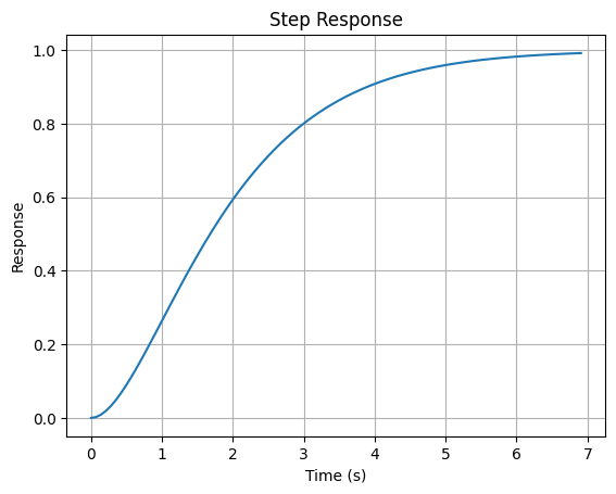
The step response of a system is its output when subjected to a step input (a sudden change from 0 to 1 at $ t = 0 $).

In the time domain, the step response $ y(t) $ of the system can be found by taking the inverse Laplace transform of:

\[Y(s) = H(s) \cdot \frac{1}{s} = \frac{1}{s(s^2 + 2s + 1)}\]

# Step Response
time, response = ctl.step_response(system)
plt.plot(time, response)
plt.title('Step Response')
plt.xlabel('Time (s)')
plt.ylabel('Response')
plt.grid()
plt.show()

3. Impulse Response

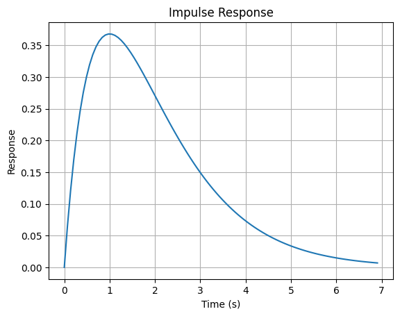
The impulse response is the output of a system when subjected to an impulse input (a Dirac delta function $ \delta(t) $).

In the Laplace domain, the impulse response $ y(t) $ is the inverse Laplace transform of:

\[Y(s) = H(s) = \frac{1}{s^2 + 2s + 1}\]

# Impulse Response
time, response = ctl.impulse_response(system)
plt.plot(time, response)
plt.title('Impulse Response')
plt.xlabel('Time (s)')
plt.ylabel('Response')
plt.grid()
plt.show()

4. Bode Plot

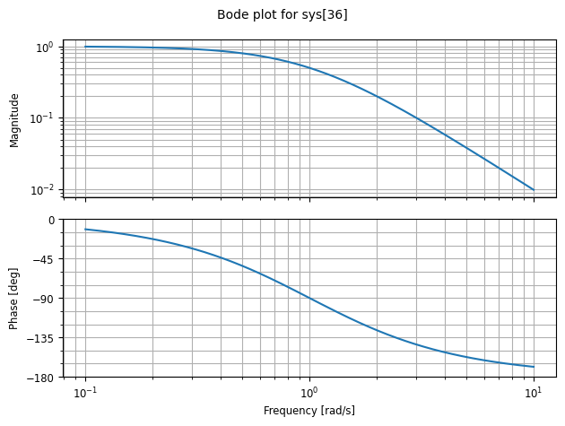
A Bode plot represents the frequency response of a system and consists of two plots:

• The magnitude plot, which shows $ \vert H(j\omega) \vert $ versus $ \omega $ (frequency).
• The phase plot, which shows $ \arg(H(j\omega)) $ versus $ \omega $.

# Bode Plot
ctl.bode(system)
plt.show()

5. PID Controller

A Proportional-Integral-Derivative (PID) controller is used to improve the response of a system. The transfer function of a PID controller is given by:

\[C(s) = K_p + \frac{K_i}{s} + K_d s\]

Where:

• $ K_p $ is the proportional gain.
• $ K_i $ is the integral gain.
• $ K_d $ is the derivative gain.

Given:

\[K_p = 1, \; K_i = 1, \; K_d = 1\]

The PID controller transfer function $ C(s) $ is:

\[C(s) = 1 + \frac{1}{s} + s = \frac{s^2 + s + 1}{s}\]

# Define and Apply PID Controller
Kp = 1
Ki = 1
Kd = 1
pid = ctl.TransferFunction([Kd, Kp, Ki], [1, 0])
closed_loop_system = ctl.feedback(pid * system)

6. Closed-Loop System with PID Controller

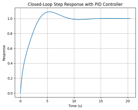
The closed-loop transfer function $ T(s) $ of the system with feedback is:

\[T(s) = \frac{C(s)H(s)}{1 + C(s)H(s)}\]

Given $ H(s) = \frac{1}{s^2 + 2s + 1} $ and $ C(s) = \frac{s^2 + s + 1}{s} $, we have:

\[T(s) = \frac{\left(\frac{s^2 + s + 1}{s}\right) \left(\frac{1}{s^2 + 2s + 1}\right)}{1 + \left(\frac{s^2 + s + 1}{s}\right) \left(\frac{1}{s^2 + 2s + 1}\right)}\]

Simplifying:

\[T(s) = \frac{s^2 + s + 1}{s(s^2 + 2s + 1) + (s^2 + s + 1)}\]

# Step Response of the Closed-Loop System with PID Controller
time, response = ctl.step_response(closed_loop_system)
plt.plot(time, response)
plt.title('Closed-Loop Step Response with PID Controller')
plt.xlabel('Time (s)')
plt.ylabel('Response')
plt.grid()
plt.show()

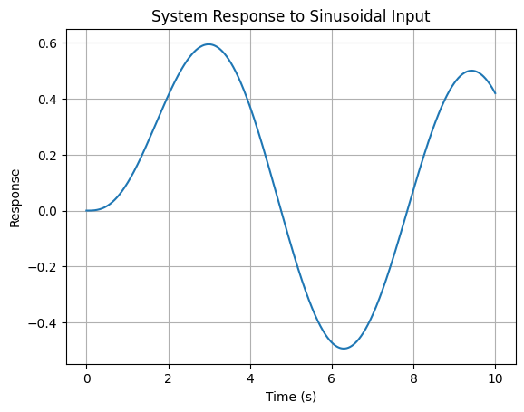
7. Sinusoidal Input Response

For a sinusoidal input $ u(t) = \sin(t) $, the system response can be analyzed by evaluating the Laplace transform and inverse Laplace transform of the product of the input and the system transfer function.

Given $ u(t) = \sin(t) $, its Laplace transform is:

\[U(s) = \frac{1}{s^2 + 1}\]

The output $ Y(s) $ is:

\[Y(s) = H(s) U(s) = \frac{1}{s^2 + 2s + 1} \cdot \frac{1}{s^2 + 1}\]

The inverse Laplace transform gives the time-domain response.

# Simulation with Sinusoidal Input
t = np.linspace(0, 10, 1000)
u = np.sin(t)
t_out, y_out, _ = signal.lsim((num, den), U=u, T=t)

plt.plot(t_out, y_out)
plt.title('System Response to Sinusoidal Input')
plt.xlabel('Time (s)')
plt.ylabel('Response')
plt.grid()
plt.show()